Tag: radial function

Kernel density estimation is a way of generating a smoothed function of density of a collection of data.

Randal Olson used Kernel density estimation to perform a statistical likelihood on the location of Waldo in the Where’s Waldo (Where’s Wally) books. Perhaps surprisingly, this didn’t reveal a random distribution, but showed that Waldo was more likely to appear in certain areas of the page.

The mathematics of kernel density estimation are closely linked to kernel smoothing, which I use a lot for my interpolation development. And since pretty much everything I do is in Grasshopper, I wanted to see if I could quickly implement KDE and make a few pretty pictures.

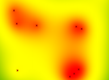
Output

Here, we can input and move a collection of points. In regions with high point density, the colour becomes more red.

And of course, making the most of the parametric capability of Grasshopper, we can move the points and get an updated Kernel Density Estimation in real time.

Grasshopper script

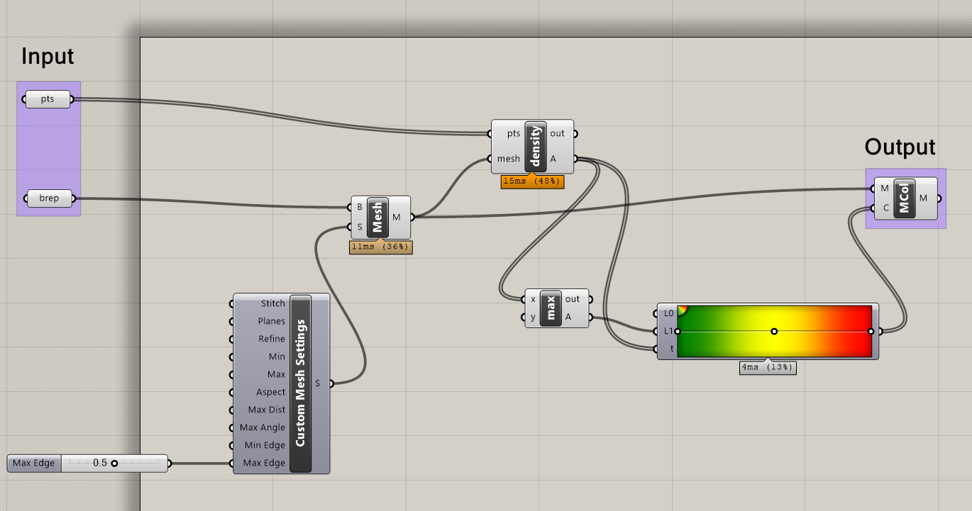
We input a mesh (or a Brep to convert to a mesh), which will provide our analysis surface for colouring later. We also input a list of data points.

A bit of C# then calculates the ‘score’ for each mesh point – or an estimation for the density over that mesh point. This returns a list of numbers. We can then colour the mesh according to these values.

The C# script – the ‘density’ component – contains the following code:

  private void RunScript(List<Point3d> pts, Mesh mesh, ref object A)
  {

    var rtnlist = new List<double>();

    foreach(var v in mesh.Vertices)
    {
      double tempval = 0;
      foreach (var pt in pts)
      {
        tempval += kernel(pt.DistanceTo(v), 0.2); //0.2 is a smoothing value - you can change this 
      }
      rtnlist.Add(tempval);
    }

    A = rtnlist;
  }

  // <Custom additional code> 

  public double kernel(double input, double factor)
  {
    return Math.Exp(-(factor * input));
  }

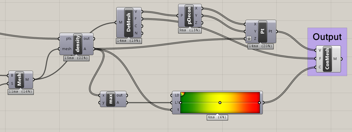
Gravity wells

The kernel density estimation can sometimes be thought of as a smoothed histogram. Another way to visualise regions of high density is to take advantage of the Z component and give our mesh some height.

To do this, I reconstructed each mesh point using the vertex score as an input for the mesh point Z component. So that the input mesh points are still easily visible, I multiplied these scores by -1. This gave a visualisation quite akin to a collection of gravity wells, the points perhaps being tiny planets floating in a 2D space.

The mesh can be modified by deconstructing the mesh and then deconstructing the points within this mesh. We then supply a modified Z value, then re-construct the mesh.