Semi-structured interviews: How many interviews are enough?

Semi-structured interviews are a useful tool for gathering qualitative information. They provide more rigour than an entirely unstructured interview, allowing the interviewer to attempt to answer a number of predefined questions and allowing common themes between interviews to be established. They are more flexible and free-flowing than questionnaires or structured interviews, allowing interviewees to diverge from an interview plan when it might provide useful information that the interviewer hadn’t anticipated asking about.

Semi-structured interviews take time

Semi-structured interviews are time-consuming to perform. Each interview is performed manually, and is usually then transcribed, analysed and codified mostly by hand. Yet, if we are using semi-structured interviews to establish patterns across a population, we must have a sufficient sample size to give us confidence in any conclusions we arrive at.

So, we want a lot of interviews as this will reinforce our findings. But we want to minimise the number of interviews so we aren’t spending weeks or months gathering and analysing data. How do we decide where the sweet spot lies?

How do people choose the right number of interviews?

The answer to this is often based on gut feeling and experience, as well as the conditions within which the research is taking place (such as number of interviewees available, time available and so on). Guides rarely provide quantified guidance. Journal articles often fail to robustly justify the number of interviews that were performed, usually citing practical limits instead.

One approach that can be taken is that of reaching a point of ‘saturation’ (Glaser & Strauss, 1967). Saturation is the point at which, after a number of interviews has been performed, it is unlikely that performing further interviews will reveal new information that hasn’t already emerged in a previous interview. Optimising the number of interviews can therefore be thought of as seeking this saturation point.

It is surprising that, given the presence of a basic knowledge of statistics in most researchers in engineering, once a social sciences technique is used in an engineering paper, the use of rigorous mathematical techniques to underpin the statistical worthiness of a series of interviews seems to be forgotten about. This deficiency has been addressed in a recent paper from Galvin (2015).

A more robust approach

Galvin attempts to answer the question of how many interviews should be performed. He is critical on the use of experience and precedence, and instead uses a range of established statistical techniques to offer guidance to the reader.

He uses the assumption that outcomes are boolean. In semi-structured interviews, this normally manifests itself as whether a theme is or isn’t present in a particular interview. This kind of data usually produces outcomes structured like “7 of the 10 interviewees mentioned saving money on bills as important when choosing to insulate their home” for example.

Without sampling the entire population, we can never be truly certain that our sample is entirely representative. But as the sample size increases, we can become increasingly confident. If (and this is a big if!) our sample is randomly selected, we can use binomial logic to say how confident we are that the results from our sample are representative of the whole population.

Why we need to take a statistical approach

This all sounds very simple, but as Galvin found, it is quite remarkable how many recent published papers exist that attempt to draw out conclusions generalised across a large population derived from tiny sample sizes, without any attempt to show that a questionably small sample size can still be relied upon to deliver a conclusive answer. Small sample sizes are to be expected with semi-structured interviews, but the time-consuming nature of this technique isn’t by itself enough justification.

What we need is a way of justifying the number of interviews that are required for our study that is robust, and that allows conclusions to be drawn from results that are statistically significant.

An equation for the number of interviews

Of interest in Galvin’s paper is therefore an equation that calculates an ideal number of interviews, given a desired confidence interval and the expected probability that a theme. The ideal number of interviewees means one that ensures that a theme held by a certain proportion of the population will have been mentioned in at least one interview. This equation to calculate the minimum number of interviews is:

equation number of semi structured interviews

P is the required confidence interval, between 0 and 1. (Galvin took a value of 0.95 throughout the paper, indicating a confidence level of 95%.) R is probability that a theme will emerge in a particular interview (e.g. the likelihood that a particular interviewee will view cost as important when insulating a home).

So, for example, if we are after a confidence level of 95%, and we guess that 70% of people view cost as important in the entire population, then we would need to conduct 3 interviews to be 95% confident that this theme will have emerged in at least one of the interviews.

Of course, the statistical reliability of this method hinges on the accuracy of our guess for R. This is unlikely to stand up to scrutiny. What may be more useful instead is if we flip the equation, and say “given that I will conduct n interviews, themes that are held by at least R% of the population are P% likely to emerge”.

The equation for this is:

semi structured interview equation

As an example, if we have conducted 10 interviews (n=10) and we will be happy with 95% confidence (P=0.95) then R=0.25, i.e. for 10 interviews, we are 95% confident that at least one person will have mentioned a theme held by at least 25% of the parent population. Or, in other words, if we run the experiment 100 times, each with a random subset of 10 interviewees, then in 95 of these, at least one person will mention a theme that is held by 25% of the parent population.

It is worth mentioning that the value of R is a function not only the proportion of the population who hold a particular theme, but also the interviewer’s skill in extracting this theme from the interviewee. While not a topic that will be dwelled upon here, this highlights the need for the interviewer to prepare and practise thoroughly to make best use of the interviews.

So, in conclusion, we have two equations which tell us in slightly different ways how many interviews we should do. If you can confidently give a lower bound estimate on R, then you can use the first equation to give the minimum number of interviews required. If you can’t estimate R, then you can use the second equation to suggest the maximum level of obscurity that a theme has amongst the population to still be exposed by your collection of interviews.

Can we estimate percentages from our interviews?

The above equation allows us to determine the minimum number of interviews to be reasonably sure that themes of interest will be mentioned in at least one interview. Once all interviews have been completed, we can expect to have a list of themes compiled from the different interviews.

Certainly, some themes will be mentioned by more than one interview. Taking the example above where 7 interviewees of 10 mention cost savings as being important, can we reasonably extrapolate this result to the whole population, and say that about 70% of the population therefore view cost savings as being important?

A basic knowledge of statistics will tell you it’s not as simple as this, and that there is a margin of error as you move from a sample to the entire population. Let’s say, after the first 10, you hypothetically carried on interviewing people until you had interviewed everybody. (In this case, this could be every homeowner in the UK!) You might have found, by the time you’d finished this gargantuan task, that in fact 18 million of 20 million homeowners thought saving money on bills was important – 90%. When you did your first 10, you were just unlucky in finding three people early on who didn’t care about bills enough to mention it.

When we take a sample, there is a probability that we will experience this ‘bad luck’ and find that our percentage from our sample is different from the percentage of the population at large. The likely difference between these percentages is the margin of error. If our sample is truly a random subset of the wider population, then we can make a statistical guess about how large this margin could be.

The trouble with small sample sizes, as is usually the case with semi-structured interviews, is that this margin is usually very large. The equation for this margin is:

wilson's score interval

Wilson’s score interval. Wilson (1904), Newcombe (1998)

p is the proportion of interviewees who mentioned a theme. z is the normal distribution z-value. If we continue using a 95% confidence interval, then z=1.96. n is the number of interviewees.

l1 and l2 are the lower and upper margins of error for p. What this equation tells us is that, if our interview tells us that p% of interviewees mention a theme, then we are 95% sure that, if we were to interview the entire population, that p would eventually converge to somewhere between l1 and l2.

If we run these numbers on a typical semi-structured interview results, where n is usually small, then the difference between l1 and l2 is large. The graph below shows results for n=3 and n=40 for a range of values of p.

margin of error for semi-structured interviews

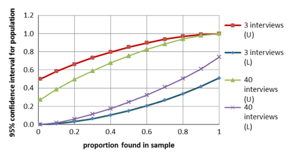
Source: Galvin (2015)

What is clear is that, typically, even for research plans with a fairly large number of interviews, the margin of error is going to be large. Too large, in fact, to be able to draw any meaningful quantified answers. If 16 of 40 interviewees (p=0.4) mention a theme, the proportion in the entire population could reasonably be anywhere between 19% and 67%.

So, the short answer is, no, you can’t usually quantify percentages from your interviews.

But in any case, this isn’t really what semi-structured interviews are for. These interviews will allow you to build a list of themes and opinions that are held by the population. Their nature allows these themes to emerge in a fluid manner in the interviews. If you are looking to quantify the occurrence of these themes, why not run a second round of surveys? Surveys are inherently rigid, but your semi-structured interviews have already allowed you to anticipate the kinds of responses people will be likely to give. And with surveys, you can issue and analyse many more, allowing you to raise that pesky n value.

References

If you found this article useful and would like to reference any information in it, then I recommend you read Galvin’s paper and pick out the information you wish to reference from there.

Galvin, R., 2015. How many interviews are enough? Do qualitative interviews in building energy consumption research produce reliable knowledge? Journal of Building Engineering, 1, pp.2–12.
Glaser, B., Strauss, A., 1967. The Discovery of Grounded Theory: Strategies for Qualitative Research, Aldine Publishing Company, New York.
Newcombe, R., 1998. Two-sided confidence intervals for the single proportion: comparison of seven methods, Stat. Med., 17, pp857–872.
Wilson, E., 1904. The Foundations of Mathematics, Bull. Am. Math. Soc. 11 (2) pp74–93.

Further reading

DiCicco-Bloom, B., Crabtree, B. F, 2006. The qualitative research interview. Medical Education, 40, pp.314-321.

Grasshopper: Calculate the Pareto front in multi-objective data in C#

A method for returning a collection of Pareto-optimal data. Pareto analysis is used in multi-objective optimisation to search for potential non-dominated solutions, i.e. solutions for which there are no solutions that perform better in every objective being assessed.

pareto-front

Input a collection of data. This data is accepted as Grasshopper’s DataTree format. The ‘tree’ contains a collection of branches. Each branch contains a list. Each list corresponds to the list of objective results corresponding to a single node.

The method sorts the input data into two DataTrees: Pareto-optimal branches and non-Pareto-optimal branches.

The algorithm is simple and unsophisticated, running in O(n2). It is fine for smaller data sets, though you may wish to investigate more sophisticated algorithms for larger datasets.

C# code to find the Pareto front

  private void RunScript(DataTree<double> data, ref object opt, ref object nonopt)
  {

    DataTree<double> optimal = new DataTree<double>();
    DataTree<double> nonoptimal = new DataTree<double>();

    //data should be a tree, where each branch is equivalent to one data point, and the length of the list is equal to the number of parameters.
    for(int n = 0; n < data.BranchCount; n++) //for each node
    {
      //check it against every other node
      //we need to find one node where every parameter is superior. if not, we have pareto optimality
      bool superiornodefound = false;
      for (int i = 0; i < data.BranchCount; i++) //check node i
      {
        bool issuperior = true;
        for(int p = 0; p < data.Branch(0).Count; p++)
        {
          if(data.Branch(i)[p] > data.Branch(n)[p])
          {
            issuperior = false;
            break;
          }
        }
        if(issuperior && i != n) superiornodefound = true;
      }
      if(superiornodefound) nonoptimal.AddRange(data.Branch(n), new GH_Path(nonoptimal.BranchCount));
      else optimal.AddRange(data.Branch(n), new GH_Path(optimal.BranchCount));
    }

    //return outputs
    opt = optimal;
    nonopt = nonoptimal;

    //grasshopper-related UI
    double optimalratio = Math.Round(100.0 * optimal.BranchCount / data.BranchCount, 1);
    Component.Message = optimalratio.ToString() + "% optimal";
    Component.Description = optimalratio.ToString() + "% of solutions are Pareto optimal.";

  }

Beware of using the UTCI approximation at extreme values

The UTCI is one of the more popular ways of estimating the perceived levels of thermal comfort in a space. In this previous post, I published some C# code that allows you to calculate the UTCI.

This code accepts inputs of air temperature, mean radiant temperature, humidity and wind velocity, and returns an equivalent perceived temperature in degC.

UTCI_scale

According to the original author here, it is only valid for certain input ranges, namely:

  • Air speed must be betwee 0.5 and 17m/s
  • MRT must be no less than 30C and no more than 70C of the air temperature
  • Air temperature must be between -50C and +50C

I have been using this UTCI code quite a lot, assuming that the model was a suitable approximation if I kept within the specified input ranges.

However, this is not always the case. While the algorithm seems to return suitable results when well within these ranges, when I started to approach the limits of these ranges (though still inside them) I noticed it is possible to generate some rather… interesting results.

Setting up a test

To test, I built a very quick document in Grasshopper. I created a graph, showing the UTCI value on the y-axis and the full range of humidity (0 to 100%) on the x-axis.

UTCI component in Grasshopper test

This seems very reasonable. A cool day, with a little warmth from the sun and a gentle breeze. The perceived temperature increases with humidity, and within a sensible range of UTCI output. Exactly what we’d expect.

Where it sometimes goes wrong

Firstly, let me say, with all sensible combinations of inputs that we’d expect to find in the real world and in our work, the UTCI returns a sensible output.

However, it is not difficult to find other combinations of inputs where the graph is a surprising shape and is clearly not right. Note that in my examples below, the inputs are still within the specified limits of the UTCI model.

Here, we can take exactly the same example, but turn up the air temperature. Look at the result when the humidity is also high.

UTCI in Grasshopper C#, erroneous result

The UTCI algorithm returns a temperature of -44C at 100% humidity – clearly not right.

Now let’s reverse the extreme values of air temperature and MRT.

UTCI Grasshopper C# erroneous result

While the result seems correct at the high end of humidity, there is a strange dip at the lower end. This isn’t so bad though, since the range of predicted UTCI values is very small (between 34.7C and 35.8C).

My advice

In most cases where values are far from the prescribed limits, the UTCI seems to return a reasonable value. In particular, it seems sensitive to extreme values of air temperature and MRT.

Particular cases seem to include when the air temperature is high (above about 40C) and when the MRT is much below the air temperature (approaching the 30C difference limit).

This isn’t conclusive, but it is more a warning to take care if your inputs are approaching the limits that the predicted UTCI could be erroneous in such cases. Most of the time, this is unlikely to affect you. But, if you are designing something like a cooling system in a hot, arab climate, or are attempting to estimate the UTCI in front of a radiant heat source, it is possible that the result might not make sense.

In particular, take care if you are implementing the UTCI in a computer program, since the computer will return an incorrect result quite happily.

UTCI: Calculation and C# code

Calculate the UTCI (Universal Thermal Climate Index) in any C# / .NET program.

What is the UTCI?

The UTCI calculates an equivalent perceived temperature based upon air temperature, radiative temperature, humidity and air movement. You may be familiar with the UTCI from weather forecasts when they say something like “the air temperature is 30C but it is going to feel more like 35C”. The UTCI is suitable as a method for calculating outdoor thermal comfort levels.

The Equivalent Temperature outputted by UTCI calculations can then be aligned to levels of thermal comfort:

UTCI_scale

Image source

Calculate the UTCI

The interaction between these four values into a single Equivalent Temperature is complex. A function, created via the method of curve-fitting, has been created by Broede as Fortran here, which is a (long!) one-line approximation of UTCI calculation. Fortran isn’t perhaps the most useful language to the average developer today, so what I have done is translate it into C# and tidy it a little by splitting up some methods.

This algorithm has been used in the outdoor comfort component in Ladybug for Grasshopper, where the Fortran code was translated into Python. An online calculator based upon this function is also available here. The source Fortran code is available here.

To use the code below, create a new class in your .NET project and copy the code below. Methods are saved as public static classes.

Example usage

Once you have added the UTCI class in your project (below), you can calculate the UTCI by calling the following method:

double utci = CalcUTCI(temp, wind, mrt, hum);

where:

  • temp: air temperature (degC)
  • wind: wind speed (m/s)
  • mrt: mean radiant temperature (degC)
  • hum: humidity ratio (0-100)

The method returns a double corresponding to the UTCI in degrees C.

Limitations

The approximation function is only valid under the following constraints:

  • Air speed must be betwee 0.5 and 17m/s
  • MRT must be no less than 30C and no more than 70C of the air temperature
  • Air temperature must be between -50C and +50C

UTCI class

    public static class C_UTCI
    {
        /*
         
             !~ UTCI, Version a 0.002, October 2009
    !~ Copyright (C) 2009  Peter Broede
    
    !~ Program for calculating UTCI Temperature (UTCI)
    !~ released for public use after termination of COST Action 730
    
    !~ replaces Version a 0.001, from September 2009

         
         * */
        /// <summary>
        /// Calculate UTCI
        /// </summary>
        /// <param name="Ta">Dry bulb air temp, degC</param>
        /// <param name="va">Air movement, m/s</param>
        /// <param name="Tmrt">Radiant temperature</param>
        /// <param name="RH">Relative humidity, 0-100%</param>
        /// <returns>UTCI 'perceived' temperature, degC. Returns double.min if input is out of range for model</returns>
        public static double CalcUTCI(double Ta, double va, double Tmrt, double RH)
        {

            if (CheckIfInputsValid(Ta, va, Tmrt, RH) != InputsChecks.Pass) return double.MinValue;
            
            double ehPa = es(Ta) * (RH / 100.0);
            double D_Tmrt = Tmrt - Ta;
            double Pa = ehPa / 10.0;//  convert vapour pressure to kPa

            #region whoa_mamma
            double UTCI_approx = Ta +
              (0.607562052) +
              (-0.0227712343) * Ta +
              (8.06470249 * Math.Pow(10, (-4))) * Ta * Ta +
              (-1.54271372 * Math.Pow(10, (-4))) * Ta * Ta * Ta +
              (-3.24651735 * Math.Pow(10, (-6))) * Ta * Ta * Ta * Ta +
              (7.32602852 * Math.Pow(10, (-8))) * Ta * Ta * Ta * Ta * Ta +
              (1.35959073 * Math.Pow(10, (-9))) * Ta * Ta * Ta * Ta * Ta * Ta +
              (-2.25836520) * va +
              (0.0880326035) * Ta * va +
              (0.00216844454) * Ta * Ta * va +
              (-1.53347087 * Math.Pow(10, (-5))) * Ta * Ta * Ta * va +
              (-5.72983704 * Math.Pow(10, (-7))) * Ta * Ta * Ta * Ta * va +
              (-2.55090145 * Math.Pow(10, (-9))) * Ta * Ta * Ta * Ta * Ta * va +
              (-0.751269505) * va * va +
              (-0.00408350271) * Ta * va * va +
              (-5.21670675 * Math.Pow(10, (-5))) * Ta * Ta * va * va +
              (1.94544667 * Math.Pow(10, (-6))) * Ta * Ta * Ta * va * va +
              (1.14099531 * Math.Pow(10, (-8))) * Ta * Ta * Ta * Ta * va * va +
              (0.158137256) * va * va * va +
              (-6.57263143 * Math.Pow(10, (-5))) * Ta * va * va * va +
              (2.22697524 * Math.Pow(10, (-7))) * Ta * Ta * va * va * va +
              (-4.16117031 * Math.Pow(10, (-8))) * Ta * Ta * Ta * va * va * va +
              (-0.0127762753) * va * va * va * va +
              (9.66891875 * Math.Pow(10, (-6))) * Ta * va * va * va * va +
              (2.52785852 * Math.Pow(10, (-9))) * Ta * Ta * va * va * va * va +
              (4.56306672 * Math.Pow(10, (-4))) * va * va * va * va * va +
              (-1.74202546 * Math.Pow(10, (-7))) * Ta * va * va * va * va * va +
              (-5.91491269 * Math.Pow(10, (-6))) * va * va * va * va * va * va +
              (0.398374029) * D_Tmrt +
              (1.83945314 * Math.Pow(10, (-4))) * Ta * D_Tmrt +
              (-1.73754510 * Math.Pow(10, (-4))) * Ta * Ta * D_Tmrt +
              (-7.60781159 * Math.Pow(10, (-7))) * Ta * Ta * Ta * D_Tmrt +
              (3.77830287 * Math.Pow(10, (-8))) * Ta * Ta * Ta * Ta * D_Tmrt +
              (5.43079673 * Math.Pow(10, (-10))) * Ta * Ta * Ta * Ta * Ta * D_Tmrt +
              (-0.0200518269) * va * D_Tmrt +
              (8.92859837 * Math.Pow(10, (-4))) * Ta * va * D_Tmrt +
              (3.45433048 * Math.Pow(10, (-6))) * Ta * Ta * va * D_Tmrt +
              (-3.77925774 * Math.Pow(10, (-7))) * Ta * Ta * Ta * va * D_Tmrt +
              (-1.69699377 * Math.Pow(10, (-9))) * Ta * Ta * Ta * Ta * va * D_Tmrt +
              (1.69992415 * Math.Pow(10, (-4))) * va * va * D_Tmrt +
              (-4.99204314 * Math.Pow(10, (-5))) * Ta * va * va * D_Tmrt +
              (2.47417178 * Math.Pow(10, (-7))) * Ta * Ta * va * va * D_Tmrt +
              (1.07596466 * Math.Pow(10, (-8))) * Ta * Ta * Ta * va * va * D_Tmrt +
              (8.49242932 * Math.Pow(10, (-5))) * va * va * va * D_Tmrt +
              (1.35191328 * Math.Pow(10, (-6))) * Ta * va * va * va * D_Tmrt +
              (-6.21531254 * Math.Pow(10, (-9))) * Ta * Ta * va * va * va * D_Tmrt +
              (-4.99410301 * Math.Pow(10, (-6))) * va * va * va * va * D_Tmrt +
              (-1.89489258 * Math.Pow(10, (-8))) * Ta * va * va * va * va * D_Tmrt +
              (8.15300114 * Math.Pow(10, (-8))) * va * va * va * va * va * D_Tmrt +
              (7.55043090 * Math.Pow(10, (-4))) * D_Tmrt * D_Tmrt +
              (-5.65095215 * Math.Pow(10, (-5))) * Ta * D_Tmrt * D_Tmrt +
              (-4.52166564 * Math.Pow(10, (-7))) * Ta * Ta * D_Tmrt * D_Tmrt +
              (2.46688878 * Math.Pow(10, (-8))) * Ta * Ta * Ta * D_Tmrt * D_Tmrt +
              (2.42674348 * Math.Pow(10, (-10))) * Ta * Ta * Ta * Ta * D_Tmrt * D_Tmrt +
              (1.54547250 * Math.Pow(10, (-4))) * va * D_Tmrt * D_Tmrt +
              (5.24110970 * Math.Pow(10, (-6))) * Ta * va * D_Tmrt * D_Tmrt +
              (-8.75874982 * Math.Pow(10, (-8))) * Ta * Ta * va * D_Tmrt * D_Tmrt +
              (-1.50743064 * Math.Pow(10, (-9))) * Ta * Ta * Ta * va * D_Tmrt * D_Tmrt +
              (-1.56236307 * Math.Pow(10, (-5))) * va * va * D_Tmrt * D_Tmrt +
              (-1.33895614 * Math.Pow(10, (-7))) * Ta * va * va * D_Tmrt * D_Tmrt +
              (2.49709824 * Math.Pow(10, (-9))) * Ta * Ta * va * va * D_Tmrt * D_Tmrt +
              (6.51711721 * Math.Pow(10, (-7))) * va * va * va * D_Tmrt * D_Tmrt +
              (1.94960053 * Math.Pow(10, (-9))) * Ta * va * va * va * D_Tmrt * D_Tmrt +
              (-1.00361113 * Math.Pow(10, (-8))) * va * va * va * va * D_Tmrt * D_Tmrt +
              (-1.21206673 * Math.Pow(10, (-5))) * D_Tmrt * D_Tmrt * D_Tmrt +
              (-2.18203660 * Math.Pow(10, (-7))) * Ta * D_Tmrt * D_Tmrt * D_Tmrt +
              (7.51269482 * Math.Pow(10, (-9))) * Ta * Ta * D_Tmrt * D_Tmrt * D_Tmrt +
              (9.79063848 * Math.Pow(10, (-11))) * Ta * Ta * Ta * D_Tmrt * D_Tmrt * D_Tmrt +
              (1.25006734 * Math.Pow(10, (-6))) * va * D_Tmrt * D_Tmrt * D_Tmrt +
              (-1.81584736 * Math.Pow(10, (-9))) * Ta * va * D_Tmrt * D_Tmrt * D_Tmrt +
              (-3.52197671 * Math.Pow(10, (-10))) * Ta * Ta * va * D_Tmrt * D_Tmrt * D_Tmrt +
              (-3.36514630 * Math.Pow(10, (-8))) * va * va * D_Tmrt * D_Tmrt * D_Tmrt +
              (1.35908359 * Math.Pow(10, (-10))) * Ta * va * va * D_Tmrt * D_Tmrt * D_Tmrt +
              (4.17032620 * Math.Pow(10, (-10))) * va * va * va * D_Tmrt * D_Tmrt * D_Tmrt +
              (-1.30369025 * Math.Pow(10, (-9))) * D_Tmrt * D_Tmrt * D_Tmrt * D_Tmrt +
              (4.13908461 * Math.Pow(10, (-10))) * Ta * D_Tmrt * D_Tmrt * D_Tmrt * D_Tmrt +
              (9.22652254 * Math.Pow(10, (-12))) * Ta * Ta * D_Tmrt * D_Tmrt * D_Tmrt * D_Tmrt +
              (-5.08220384 * Math.Pow(10, (-9))) * va * D_Tmrt * D_Tmrt * D_Tmrt * D_Tmrt +
              (-2.24730961 * Math.Pow(10, (-11))) * Ta * va * D_Tmrt * D_Tmrt * D_Tmrt * D_Tmrt +
              (1.17139133 * Math.Pow(10, (-10))) * va * va * D_Tmrt * D_Tmrt * D_Tmrt * D_Tmrt +
              (6.62154879 * Math.Pow(10, (-10))) * D_Tmrt * D_Tmrt * D_Tmrt * D_Tmrt * D_Tmrt +
              (4.03863260 * Math.Pow(10, (-13))) * Ta * D_Tmrt * D_Tmrt * D_Tmrt * D_Tmrt * D_Tmrt +
              (1.95087203 * Math.Pow(10, (-12))) * va * D_Tmrt * D_Tmrt * D_Tmrt * D_Tmrt * D_Tmrt +
              (-4.73602469 * Math.Pow(10, (-12))) * D_Tmrt * D_Tmrt * D_Tmrt * D_Tmrt * D_Tmrt * D_Tmrt +
              (5.12733497) * Pa +
              (-0.312788561) * Ta * Pa +
              (-0.0196701861) * Ta * Ta * Pa +
              (9.99690870 * Math.Pow(10, (-4))) * Ta * Ta * Ta * Pa +
              (9.51738512 * Math.Pow(10, (-6))) * Ta * Ta * Ta * Ta * Pa +
              (-4.66426341 * Math.Pow(10, (-7))) * Ta * Ta * Ta * Ta * Ta * Pa +
              (0.548050612) * va * Pa +
              (-0.00330552823) * Ta * va * Pa +
              (-0.00164119440) * Ta * Ta * va * Pa +
              (-5.16670694 * Math.Pow(10, (-6))) * Ta * Ta * Ta * va * Pa +
              (9.52692432 * Math.Pow(10, (-7))) * Ta * Ta * Ta * Ta * va * Pa +
              (-0.0429223622) * va * va * Pa +
              (0.00500845667) * Ta * va * va * Pa +
              (1.00601257 * Math.Pow(10, (-6))) * Ta * Ta * va * va * Pa +
              (-1.81748644 * Math.Pow(10, (-6))) * Ta * Ta * Ta * va * va * Pa +
              (-1.25813502 * Math.Pow(10, (-3))) * va * va * va * Pa +
              (-1.79330391 * Math.Pow(10, (-4))) * Ta * va * va * va * Pa +
              (2.34994441 * Math.Pow(10, (-6))) * Ta * Ta * va * va * va * Pa +
              (1.29735808 * Math.Pow(10, (-4))) * va * va * va * va * Pa +
              (1.29064870 * Math.Pow(10, (-6))) * Ta * va * va * va * va * Pa +
              (-2.28558686 * Math.Pow(10, (-6))) * va * va * va * va * va * Pa +
              (-0.0369476348) * D_Tmrt * Pa +
              (0.00162325322) * Ta * D_Tmrt * Pa +
              (-3.14279680 * Math.Pow(10, (-5))) * Ta * Ta * D_Tmrt * Pa +
              (2.59835559 * Math.Pow(10, (-6))) * Ta * Ta * Ta * D_Tmrt * Pa +
              (-4.77136523 * Math.Pow(10, (-8))) * Ta * Ta * Ta * Ta * D_Tmrt * Pa +
              (8.64203390 * Math.Pow(10, (-3))) * va * D_Tmrt * Pa +
              (-6.87405181 * Math.Pow(10, (-4))) * Ta * va * D_Tmrt * Pa +
              (-9.13863872 * Math.Pow(10, (-6))) * Ta * Ta * va * D_Tmrt * Pa +
              (5.15916806 * Math.Pow(10, (-7))) * Ta * Ta * Ta * va * D_Tmrt * Pa +
              (-3.59217476 * Math.Pow(10, (-5))) * va * va * D_Tmrt * Pa +
              (3.28696511 * Math.Pow(10, (-5))) * Ta * va * va * D_Tmrt * Pa +
              (-7.10542454 * Math.Pow(10, (-7))) * Ta * Ta * va * va * D_Tmrt * Pa +
              (-1.24382300 * Math.Pow(10, (-5))) * va * va * va * D_Tmrt * Pa +
              (-7.38584400 * Math.Pow(10, (-9))) * Ta * va * va * va * D_Tmrt * Pa +
              (2.20609296 * Math.Pow(10, (-7))) * va * va * va * va * D_Tmrt * Pa +
              (-7.32469180 * Math.Pow(10, (-4))) * D_Tmrt * D_Tmrt * Pa +
              (-1.87381964 * Math.Pow(10, (-5))) * Ta * D_Tmrt * D_Tmrt * Pa +
              (4.80925239 * Math.Pow(10, (-6))) * Ta * Ta * D_Tmrt * D_Tmrt * Pa +
              (-8.75492040 * Math.Pow(10, (-8))) * Ta * Ta * Ta * D_Tmrt * D_Tmrt * Pa +
              (2.77862930 * Math.Pow(10, (-5))) * va * D_Tmrt * D_Tmrt * Pa +
              (-5.06004592 * Math.Pow(10, (-6))) * Ta * va * D_Tmrt * D_Tmrt * Pa +
              (1.14325367 * Math.Pow(10, (-7))) * Ta * Ta * va * D_Tmrt * D_Tmrt * Pa +
              (2.53016723 * Math.Pow(10, (-6))) * va * va * D_Tmrt * D_Tmrt * Pa +
              (-1.72857035 * Math.Pow(10, (-8))) * Ta * va * va * D_Tmrt * D_Tmrt * Pa +
              (-3.95079398 * Math.Pow(10, (-8))) * va * va * va * D_Tmrt * D_Tmrt * Pa +
              (-3.59413173 * Math.Pow(10, (-7))) * D_Tmrt * D_Tmrt * D_Tmrt * Pa +
              (7.04388046 * Math.Pow(10, (-7))) * Ta * D_Tmrt * D_Tmrt * D_Tmrt * Pa +
              (-1.89309167 * Math.Pow(10, (-8))) * Ta * Ta * D_Tmrt * D_Tmrt * D_Tmrt * Pa +
              (-4.79768731 * Math.Pow(10, (-7))) * va * D_Tmrt * D_Tmrt * D_Tmrt * Pa +
              (7.96079978 * Math.Pow(10, (-9))) * Ta * va * D_Tmrt * D_Tmrt * D_Tmrt * Pa +
              (1.62897058 * Math.Pow(10, (-9))) * va * va * D_Tmrt * D_Tmrt * D_Tmrt * Pa +
              (3.94367674 * Math.Pow(10, (-8))) * D_Tmrt * D_Tmrt * D_Tmrt * D_Tmrt * Pa +
              (-1.18566247 * Math.Pow(10, (-9))) * Ta * D_Tmrt * D_Tmrt * D_Tmrt * D_Tmrt * Pa +
              (3.34678041 * Math.Pow(10, (-10))) * va * D_Tmrt * D_Tmrt * D_Tmrt * D_Tmrt * Pa +
              (-1.15606447 * Math.Pow(10, (-10))) * D_Tmrt * D_Tmrt * D_Tmrt * D_Tmrt * D_Tmrt * Pa +
              (-2.80626406) * Pa * Pa +
              (0.548712484) * Ta * Pa * Pa +
              (-0.00399428410) * Ta * Ta * Pa * Pa +
              (-9.54009191 * Math.Pow(10, (-4))) * Ta * Ta * Ta * Pa * Pa +
              (1.93090978 * Math.Pow(10, (-5))) * Ta * Ta * Ta * Ta * Pa * Pa +
              (-0.308806365) * va * Pa * Pa +
              (0.0116952364) * Ta * va * Pa * Pa +
              (4.95271903 * Math.Pow(10, (-4))) * Ta * Ta * va * Pa * Pa +
              (-1.90710882 * Math.Pow(10, (-5))) * Ta * Ta * Ta * va * Pa * Pa +
              (0.00210787756) * va * va * Pa * Pa +
              (-6.98445738 * Math.Pow(10, (-4))) * Ta * va * va * Pa * Pa +
              (2.30109073 * Math.Pow(10, (-5))) * Ta * Ta * va * va * Pa * Pa +
              (4.17856590 * Math.Pow(10, (-4))) * va * va * va * Pa * Pa +
              (-1.27043871 * Math.Pow(10, (-5))) * Ta * va * va * va * Pa * Pa +
              (-3.04620472 * Math.Pow(10, (-6))) * va * va * va * va * Pa * Pa +
              (0.0514507424) * D_Tmrt * Pa * Pa +
              (-0.00432510997) * Ta * D_Tmrt * Pa * Pa +
              (8.99281156 * Math.Pow(10, (-5))) * Ta * Ta * D_Tmrt * Pa * Pa +
              (-7.14663943 * Math.Pow(10, (-7))) * Ta * Ta * Ta * D_Tmrt * Pa * Pa +
              (-2.66016305 * Math.Pow(10, (-4))) * va * D_Tmrt * Pa * Pa +
              (2.63789586 * Math.Pow(10, (-4))) * Ta * va * D_Tmrt * Pa * Pa +
              (-7.01199003 * Math.Pow(10, (-6))) * Ta * Ta * va * D_Tmrt * Pa * Pa +
              (-1.06823306 * Math.Pow(10, (-4))) * va * va * D_Tmrt * Pa * Pa +
              (3.61341136 * Math.Pow(10, (-6))) * Ta * va * va * D_Tmrt * Pa * Pa +
              (2.29748967 * Math.Pow(10, (-7))) * va * va * va * D_Tmrt * Pa * Pa +
              (3.04788893 * Math.Pow(10, (-4))) * D_Tmrt * D_Tmrt * Pa * Pa +
              (-6.42070836 * Math.Pow(10, (-5))) * Ta * D_Tmrt * D_Tmrt * Pa * Pa +
              (1.16257971 * Math.Pow(10, (-6))) * Ta * Ta * D_Tmrt * D_Tmrt * Pa * Pa +
              (7.68023384 * Math.Pow(10, (-6))) * va * D_Tmrt * D_Tmrt * Pa * Pa +
              (-5.47446896 * Math.Pow(10, (-7))) * Ta * va * D_Tmrt * D_Tmrt * Pa * Pa +
              (-3.59937910 * Math.Pow(10, (-8))) * va * va * D_Tmrt * D_Tmrt * Pa * Pa +
              (-4.36497725 * Math.Pow(10, (-6))) * D_Tmrt * D_Tmrt * D_Tmrt * Pa * Pa +
              (1.68737969 * Math.Pow(10, (-7))) * Ta * D_Tmrt * D_Tmrt * D_Tmrt * Pa * Pa +
              (2.67489271 * Math.Pow(10, (-8))) * va * D_Tmrt * D_Tmrt * D_Tmrt * Pa * Pa +
              (3.23926897 * Math.Pow(10, (-9))) * D_Tmrt * D_Tmrt * D_Tmrt * D_Tmrt * Pa * Pa +
              (-0.0353874123) * Pa * Pa * Pa +
              (-0.221201190) * Ta * Pa * Pa * Pa +
              (0.0155126038) * Ta * Ta * Pa * Pa * Pa +
              (-2.63917279 * Math.Pow(10, (-4))) * Ta * Ta * Ta * Pa * Pa * Pa +
              (0.0453433455) * va * Pa * Pa * Pa +
              (-0.00432943862) * Ta * va * Pa * Pa * Pa +
              (1.45389826 * Math.Pow(10, (-4))) * Ta * Ta * va * Pa * Pa * Pa +
              (2.17508610 * Math.Pow(10, (-4))) * va * va * Pa * Pa * Pa +
              (-6.66724702 * Math.Pow(10, (-5))) * Ta * va * va * Pa * Pa * Pa +
              (3.33217140 * Math.Pow(10, (-5))) * va * va * va * Pa * Pa * Pa +
              (-0.00226921615) * D_Tmrt * Pa * Pa * Pa +
              (3.80261982 * Math.Pow(10, (-4))) * Ta * D_Tmrt * Pa * Pa * Pa +
              (-5.45314314 * Math.Pow(10, (-9))) * Ta * Ta * D_Tmrt * Pa * Pa * Pa +
              (-7.96355448 * Math.Pow(10, (-4))) * va * D_Tmrt * Pa * Pa * Pa +
              (2.53458034 * Math.Pow(10, (-5))) * Ta * va * D_Tmrt * Pa * Pa * Pa +
              (-6.31223658 * Math.Pow(10, (-6))) * va * va * D_Tmrt * Pa * Pa * Pa +
              (3.02122035 * Math.Pow(10, (-4))) * D_Tmrt * D_Tmrt * Pa * Pa * Pa +
              (-4.77403547 * Math.Pow(10, (-6))) * Ta * D_Tmrt * D_Tmrt * Pa * Pa * Pa +
              (1.73825715 * Math.Pow(10, (-6))) * va * D_Tmrt * D_Tmrt * Pa * Pa * Pa +
              (-4.09087898 * Math.Pow(10, (-7))) * D_Tmrt * D_Tmrt * D_Tmrt * Pa * Pa * Pa +
              (0.614155345) * Pa * Pa * Pa * Pa +
              (-0.0616755931) * Ta * Pa * Pa * Pa * Pa +
              (0.00133374846) * Ta * Ta * Pa * Pa * Pa * Pa +
              (0.00355375387) * va * Pa * Pa * Pa * Pa +
              (-5.13027851 * Math.Pow(10, (-4))) * Ta * va * Pa * Pa * Pa * Pa +
              (1.02449757 * Math.Pow(10, (-4))) * va * va * Pa * Pa * Pa * Pa +
              (-0.00148526421) * D_Tmrt * Pa * Pa * Pa * Pa +
              (-4.11469183 * Math.Pow(10, (-5))) * Ta * D_Tmrt * Pa * Pa * Pa * Pa +
              (-6.80434415 * Math.Pow(10, (-6))) * va * D_Tmrt * Pa * Pa * Pa * Pa +
              (-9.77675906 * Math.Pow(10, (-6))) * D_Tmrt * D_Tmrt * Pa * Pa * Pa * Pa +
              (0.0882773108) * Pa * Pa * Pa * Pa * Pa +
              (-0.00301859306) * Ta * Pa * Pa * Pa * Pa * Pa +
              (0.00104452989) * va * Pa * Pa * Pa * Pa * Pa +
              (2.47090539 * Math.Pow(10, (-4))) * D_Tmrt * Pa * Pa * Pa * Pa * Pa +
              (0.00148348065) * Pa * Pa * Pa * Pa * Pa * Pa;
            #endregion

            return UTCI_approx;
        }


        /// <summary>
        /// Calc saturation vapour pressure
        /// </summary>
        /// <param name="ta">Input air temperature, degC</param>
        /// <returns></returns>
        private static double es(double ta)
        {
            //calculates saturation vapour pressure over water in hPa for input air temperature (ta) in celsius according to:
            //Hardy, R.; ITS-90 Formulations for Vapor Pressure, Frostpoint Temperature, Dewpoint Temperature and Enhancement Factors in the Range -100 to 100 °C; 
            //Proceedings of Third International Symposium on Humidity and Moisture; edited by National Physical Laboratory (NPL), London, 1998, pp. 214-221
            //http://www.thunderscientific.com/tech_info/reflibrary/its90formulas.pdf (retrieved 2008-10-01)

            double[] g = new double[] { -2836.5744, -6028.076559, 19.54263612, -0.02737830188, 0.000016261698, ((double)(7.0229056 * Math.Pow(10, -10))), ((double)(-1.8680009 * Math.Pow(10, -13))) };
            double tk = ta + 273.15;
            double es = 2.7150305 * Math.Log(tk);
            //for count, i in enumerate(g):
            for (int count = 0; count < g.Length; count++)
            {
                double i = g[count];
                es = es + (i * Math.Pow(tk, (count - 2)));
            }
            es = Math.Exp(es) * 0.01;
            return es;
        }


        public static InputsChecks CheckIfInputsValid(double Ta, double va, double Tmrt, double hum)
        {

        if (Ta < -50.0 || Ta > 50.0) return InputsChecks.Temp_OutOfRange;
        if (Tmrt-Ta < -30.0 || Tmrt-Ta > 70.0) return InputsChecks.Large_Gap_Between_Trmt_Ta;
        if (va < 0.5) return InputsChecks.WindSpeed_Too_Low;
        if (va > 17) return InputsChecks.WindSpeed_TooHigh;
        return InputsChecks.Pass;
        }

        public enum InputsChecks { Temp_OutOfRange, Large_Gap_Between_Trmt_Ta, WindSpeed_Too_Low, WindSpeed_TooHigh, Pass, Unknown }
       

    }

References

Papers presenting the UTCI:

  • UTCI poster, 13th International Conference on Environmental Ergonomics, Boston, Massachusetts, USA, 2-7 Aug 2009

Papers utilising the UTCI:

  • Journal article Sookuk Park, Stanton E. Tuller, Myunghee Jo, Application of Universal Thermal Climate Index (UTCI) for microclimatic analysis in urban thermal environments, Landscape and Urban Planning, Volume 125, May 2014, Pages 146-155
  • Journal article Katerina Pantavou, George Theoharatos, Mattheos Santamouris, Dimosthenis Asimakopoulos, Outdoor thermal sensation of pedestrians in a Mediterranean climate and a comparison with UTCI, Building and Environment, Volume 66, August 2013, Pages 82-95, ISSN 0360-1323, http://dx.doi.org/10.1016/j.buildenv.2013.02.014.

I presented at CIBSE Technical Symposium 2015

Last week I presented a software tool I have been developing in collaboration with Smart Space at BuroHappold called SmartBuildingAnalyser. CIBSE Technical Symposium is a meeting of academic and industrial developments which aim to look at the latest advances in tools and methodologies for the many aspects of building environmental design. This year, the conference was held at UCL in London.

James Ramsden presenting SmartBuildingAnalyser at CIBSE Technical Symposium 2015

Presentation abstract

The paper and presentation set out the problem of the complexity and contradictions that arise as we try to design the ‘perfect’ building. I attempted to argue that, since there is no such thing as a perfect building, trade-offs are inevitable, and that the best way to get the best combination of trade-offs is to have a better understanding of how different options perform. Currently the tools available for ‘optioneering’ are not powerful enough to generate this data for a wide range of options in a reasonable amount of time.

SmartBuildingAnalyser is a collection of components currently under development for Grasshopper that help to leverage the power of Grasshopper for the specific task of streamlining the parametric building design and analysis process. In the presentation, I showed how these components generated options for a number of projects in BuroHappold to expose how the sensitivity of building performance with respect to the changing of certain design parameters.

Many of the posts on this site, especially the ‘hints and tips’ style posts on Grasshopper, were written as part of the various pieces of development towards SBA. I’m still a fair way off a public release of SBA, but it’s well on its way, and hopefully the presentation will have generated enough interest to provide the links necessary for further work.

How did it go?

I have given a small number of presentations before as part of my work, mostly internal to BuroHappold but most notably to COLEB in ETH, Zurich last year. The CIBSE presentation was, by quite a margin, the most significant and impactful presentation I have given to date – I was fortunate to have an enthusiastic and prolific audience of perhaps 50 delegates. While it was rather intimidating when waiting to give my speech, I needn’t have worried – the audience were receptive and were keen to pass on their feedback and discussion points later on in the day. (Thank you to everyone who did this – your feedback and insights are very valuable to me!)

Every experience like this is a learning process, and especially at this CIBSE event where most participants aren’t programmers of any description, it’s good practice to learn to explain my work in an accessible way. One key failing is that I didn’t quite explain where in the design process my tool lies. The gap in software I have identified is in the transition between concept and detailed design stages. I am not trying to compete with ‘architect’ conceptual tools such as Sefaira or Vasari, nor have I developed a tool that provides the level of detail (and associated time cost) of detailing that comes with Dynamo, but I am aiming for the space between, where the design has progressed to the point where engineering questions are being asked of a building where the form is still still subject to a significant amount of uncertainty.

Download paper and presentation

I have uploaded the paper to academia.edu.

The full presentation with videos is available from this site here.

Where do I publish my first scientific paper?

Coming up to two years in my research journey in my Engineering Doctorate, the time is already overdue for me to publish my first paper. Scientific papers that want to be held in the highest esteem should be published in a peer-reviewed journal.

With support from my supervisor and colleagues, I am now starting to look into the process. With a few ideas on the go, each I believe worthy of eventually becoming a paper, a key question is which journal to target.

An obvious starting point is to look at the literature related to my work, and see where they have been published. Scanning through my Mendeley library, four journals seem to stand out:

Reading through the scope of these journals reveals a lot of overlap, which doesn’t do much for helping to narrow down my options. I can’t necessarily just submit a paper to all of them, hoping for one of them to accept my paper – this simply isn’t allowed. So I need to be selective about which journal I submit my paper to.

Impact factor

Not all journals are created equally, and naturally I want to choose a journal with a strong reputation. A key measure of journal reputation is the Impact Factor, which is basically the average number of citations each paper in the journal receives. SciJournal provides a quick way of looking up the Impact Factor for various journals in recent years, so I took a look for the four above:

2008 2009 2010 2011 2012 2013-2014
Energy and Buildings 1.59 1.593 2.041 2.386 2.679 2.465
Building and Environment 1.192 1.797 2.129 2.4 2.43 2.7
Automation in construction 1.664 1.372 1.311 1.5 1.82 1.822
Energy 1.712 2.952 3.565 3.487 3.651 4.159

‘Energy’ clearly stands out as the journal with the strongest impact, but it is also the most general of the four journals. The most impactful journals may be more competitive, and with the review process taking many months, I want to minimise the chances of my paper being rejected. While I want to aim high, it’s better to have a paper in a middling journal than not published at all.

SJR

Another interesting site to browse is SCImago Journal and Country Rank, which provides more in-depth information and rankings. Looking at the Buildings and Construction category, Energy and Buildings comes 7th based on their SJR metric. (Note that it’s a Spanish site, so commas are decimal points, and full stops are thousand separators!) The 6 superior journals aren’t relevant, so this journal is looking promising. ‘Energy’ doesn’t appear in this category, as expected. ‘Building and Environment’ comes 13th, while ‘Automation in Construction’ trails in at 18th.

The advantage of scanning tables like this is that it can expose journals that may have been missed in the literature review. Building Research & Information comes in at 17th on this SJR table, having relevance to me in terms of building performance. The Journal of Building Performance Simulation is at 24th, but it is a newer journal and is rising quite quickly year on year.

Conference report: COLEB 2014

ETH Zurich

What is COLEB?

COLEB (Computational Optimisation of Low Energy Buildings) is a 2-day workshop and conference held at ETH in Zurich on 6-7 March 2014. The various topics focused on the development and application of computational methods and algorithms into improving various aspects of building design. Some specific areas included:

  • Design optimisation (Using algorithms to improve aspects of building design)
  • Control optimisation (Such as improving the scheduling algorithms of HVAC)
  • Distributed energy systems (Including managing the issues with storage, load management and unplanned outages)

The event was co-organised and ran by Dr. Ralph Evins, a graduate of the Systems Centre and my EngD predecessor at Buro Happold. It was kindly sponsored by the Chair of Building Physics at ETH Zurich and the Swiss Competence Centre – Energy and Mobility Project “Integration of Decentralized Energy Adaptive Systems for cities”.

This is the first iteration of COLEB, and unfortunately it was never intended to be repeated exactly in its current form. However, there is talk of another COLEB workshop possibly being organised in the future. Watch this space!

Why did I go?

I have already attended a conference – FutureBuild at the University of Bath – but did not present – it was far too early in my research, and in any case the theme seemed too far removed from my own work. But COLEB – with its intention of looking at the latest modelling and optimisation methods as applied to efficient building design – seemed perfect for me as a place to give my first presentation.

Your first conference presentation?? What was it like?

In form true to myself, the presentation was only finished mere days before the workshop, and I was still writing my speech for it in the airport. Practising in the mirror in the hotel the night before, I finally had it nailed.

But actually getting up to do the presentation in front of around 30 people, I introduced myself, got on to the first slide, and immediately forgot every word! So, instead of my careful plan, I just started talking. It was roughly in line with my speech but certainly not what I’d rehearsed. In the end, it was a very free-form speech and it was, I think, quite successful, and even though I didn’t stick to my planned speech, the practice was still essential for me being relatively comfortable with it.

How was the rest of it?

As the only participant with a primarily industrial focus to my research, I did hold somewhat of a special position in the conference. There were some very interesting ideas all round, though there was always a voice in the back of my mind judging each speech on the practical and commercial viability, something I think to some extent sets industrial and academic minds apart. But this blue-sky approach is perhaps something we need to be more confident of embracing in industry – we can be too quick to dismiss an idea if we can’t foresee a safe return.
One key benefit of going to conferences is the opportunity to network. COLEB was formed partially as a result of the community of those who attend the likes of the BSO conferences, and there was interest among a number of the participants in creating and attending a second COLEB next year. Specifically with regards to individuals, business cards were exchanged and I have made a number of follow-up commitments with participants, which hopefully may turn into something very interesting.

Seems interesting! Where can I learn more?

You can visit the website here. The website includes copies of my presentation and paper, as well as for the other attendees. You can also contact me directly if you have any questions 🙂

List of building simulation conferences

A growing list of conferences to do with optimisation, structural/environmental and holistic building design and anything else of interest…

IBPSA Building Simulation Conference

International Building Performance Simulation Association. Started 1985, held every 2 years, 14 conferences held so far. Various international locations.

  • When: 2015
  • Where: Hyderabad, India

http://www.ibpsa.org/?page_id=44

http://www.bs2015.in/index.html

Conference papers/proceedings for IBPSA can be found at http://www.ibpsa.org/?page_id=349

IBPSA England – Building Simulation and Optimization

One event held so far, next in 2014. Abstract submission due this week, paper submission 16th Jan. Early bird tickets deadline 16th April.

  • When: 23-24 June 2013
  • Where: UCL, London

http://www.bso14.org/

IStructE – 16th Young Researchers Conference

Focused towards engineers in years 2 and 3 of their research, for those with less than 3 years’ research experience, and under 30 years old. 1st year students are not expected to present but are encouraged to attend. Free entry to registered delegates. Deadlines: 22nd Nov (1st year); 1st Nov (2/3 year)

  • When: 5 March 2014
  • Where: London

http://www.istructe.org/events-awards/conference-and-lectures/young-researchers-conference

GeCo In The Rockies

  • When: 22-26 Sept 2014
  • Where: Grand Junction, Colorado

http://www.gecointherockies.org/

Evo*

“The leading European event on bio-inspired computation” – since 1998

  • When: 23-25 April 2014
  • Where: Granada, Spain

Umbrella event for a number of conferences:

  • EuroGP – 17th International Conference on Genetic Programming
  • EvoCOP – 14th International Conference on Evolutionary Computation in Combinatorial Optimization
  • EvoBio – 12th International Conference on Evolutionary Computation, Machine Learning and Data Mining in Computational Biology
  • EvoMUSART – 3rd International Conference on evolutionary and biologically inspired music, sound, art and design
  • EvoApplications – 16th Annual Conference on the applications of evolutionary computation. Includes many sub-conferences, such as EvoComplex (evolutionary algorithms and complex systems), EvoHOT (bio-inspired heuristics for design automation)… see http://www.evostar.org/flyer/evo2014_granada_opt.pdf


http://www.evostar.org/

Filming: Day 2 (22nd Aug)

This article continues on from filming day 1.

The second day of the film course was when we would take our storyboards from the 6th August, have some fun in front of a camera, and turn our ideas into professionally edited short films. The morning was scheduled for filming, and with barely time to eat, the plan was to get the film sent back to Uni and stitch the clips together into something we could be proud of. As if that didn’t sound tight enough, the weather was good and conditions were right for us to record two films. Continue reading Filming: Day 2 (22nd Aug)